
Reinforcement Learning for Algorithmic Trading
Creating a Prototype Multi-Stock Environment on QuantConnect

Reinforcement Learning for Algorithmic Trading: Creating a Prototype Multi-Stock Environment on QuantConnect
Disclaimer: The information presented in this article is for educational purposes only and does not constitute financial advice. I am not affiliated with QuantConnect or any other trading platform, and the algorithm discussed should undergo significant refinement and testing before any live trading implementation.
In recent years, the application of reinforcement learning (RL) in algorithmic trading has gained considerable attention. The ability to dynamically adapt to market conditions through training an agent to make trading decisions based on reward signals is an intriguing concept. This article delves into a specific implementation of a reinforcement learning algorithm using Deep Q-Networks (DQN) within a multi-stock trading environment on the QuantConnect platform.
Understanding Deep Q-Networks (DQN)
DQN is a type of reinforcement learning algorithm that combines Q-learning with deep neural networks. It addresses the challenge of high-dimensional state spaces common in trading by using a neural network to approximate the Q-value function. The Q-value represents the expected utility of taking a particular action in a given state, allowing the agent to learn optimal policies over time.
In the context of trading, states could be defined by various indicators, such as moving averages and momentum indicators, while actions could be to buy, sell, or hold a stock. The agent learns from the environment by interacting with it and receiving feedback in the form of rewards based on the profit or loss incurred from its actions.
The Multi-Stock Trading Algorithm
The following code snippet demonstrates an implementation of the Ensemble Regime Detection algorithm using the DQN architecture. This algorithm dynamically selects stocks based on market conditions and employs a reinforcement learning model to make trading decisions.
import gym
import numpy as np
from AlgorithmImports import *
from stable_baselines3 import DQN
from datetime import timedelta

class MultiStockTrading(QCAlgorithm):

    def Initialize(self):
        self.SetStartDate(2024, 1, 1)
        self._num_fine = 3
        self._num_coarse = 10

self.SetPortfolioConstruction(EqualWeightingPortfolioConstructionModel(timedelta(minutes=5)))
        self.Settings.RebalancePortfolioOnInsightChanges = False
        self.SetWarmup(150)  # Warm up for technical indicators

        self.AddUniverse(self._coarse_selection_function, self._fine_selection_function)
        self.last_training_time = self.StartDate

    def _coarse_selection_function(self, coarse):
        '''Select securities with highest dollar volume'''
        selected = sorted([x for x in coarse if x.HasFundamentalData and x.Price > 5],
                          key=lambda x: x.DollarVolume, reverse=True)
        return [x.Symbol for x in selected[:self._num_coarse]]

    def _fine_selection_function(self, fine):
        '''Select securities with highest market cap'''
        selected = sorted(fine, key=lambda f: f.MarketCap, reverse=True)
        return [x.Symbol for x in selected[:self._num_fine]]
Dynamic Trading Environment
To enable the agent to interact with the trading environment, we create a custom TradingEnv class that encapsulates the trading logic and defines the state and action spaces.
class TradingEnv(gym.Env):
    def __init__(self, security):
        super(TradingEnv, self).__init__()
        self.security = security
        self.trading_cost = 0.01
        self.current_step = 0
        self.returns = []
        self.action_space = gym.spaces.Discrete(3)  # Hold, Buy, Sell
        self.observation_space = gym.spaces.Box(low=-np.inf, high=np.inf, shape=(6,), dtype=np.float32)  # 6 features

    def reset(self):
        self.current_step = 0
        self.returns = []
        return self._get_observation()

    def step(self, action):
        current_roc = self.security.roc.Current.Value
        reward = 0
        if action == 1:  # Buy action
            reward = current_roc - self.trading_cost
        elif action == 2:  # Sell action
            reward = -current_roc - self.trading_cost

        self.returns.append(reward)
        self.current_step += 1

        done = self.current_step >= self.security.roc.Window.Count

        if done:
            returns_array = np.array(self.returns)
            sharpe_ratio = (returns_array.mean() - 0.01) / returns_array.std() if returns_array.std() > 0 else 0
            reward = sharpe_ratio

        return self._get_observation(), reward, done, {}

    def _get_observation(self):
        return np.array([
            self.security.roc.Current.Value,
            self.security.sma.Current.Value,
            self.security.ema.Current.Value,
            self.security.rsi.Current.Value,
            self.security.bbands.UpperBand.Current.Value - self.security.bbands.LowerBand.Current.Value,  # BB width
            self.security.atr.Current.Value
        ]).astype(np.float32)
Trading Strategy Implementation
In the OnConsolidated method, the DQN model is utilized to make predictions based on the current state of the stock. It emits insights to guide trading actions.
def OnConsolidated(self, _, bar):
    security = self.Securities[bar.Symbol]
    if security.sma.IsReady and security.rsi.IsReady:
        # Prepare feature set
        features = np.array([
            security.roc.Current.Value,
            security.sma.Current.Value,
            security.ema.Current.Value,
            security.rsi.Current.Value,
            security.bbands.UpperBand.Current.Value - security.bbands.LowerBand.Current.Value,  # Bollinger Bands width
            security.atr.Current.Value
        ]).reshape(1, -1)

        # DQN model prediction
        action, _states = security.dqn_model.predict(features)

        # Define insights based on the action
        direction = InsightDirection.FLAT
        if action == 1:  # Buy/Long
            direction = InsightDirection.UP
        elif action == 2:  # Sell/Short
            direction = InsightDirection.DOWN

        self.EmitInsights(Insight.Price(bar.Symbol, timedelta(minutes=5), direction))
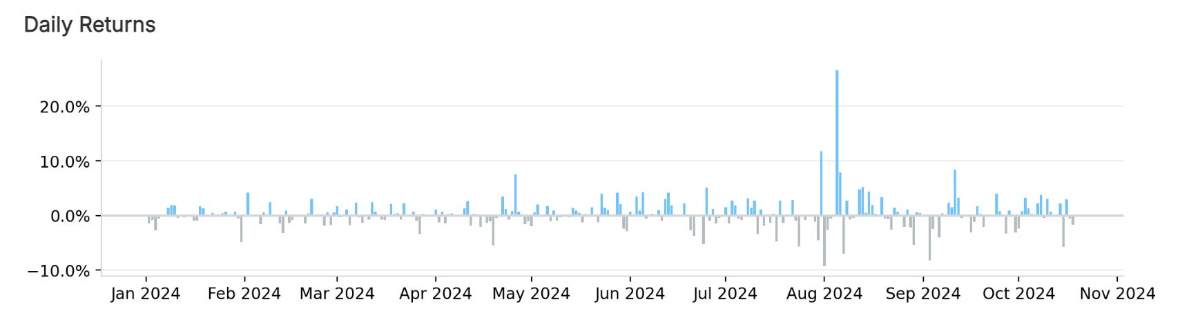
Performance Overview
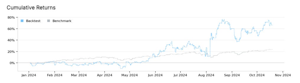
After launching the algorithm, it produced notable results during its testing period, starting on January 1, 2024. Here are some key performance metrics:
Sharpe Ratio: 1.444
Compounding Annual Return: 88.74%
Maximum Drawdown: 22.70%
Total Orders: 6,975
Net Profit: 66.21%
Win Rate: 47%
Loss Rate: 53%
These metrics reflect a robust strategy capable of achieving high returns, though it also displays considerable volatility, as indicated by the drawdown percentage.
Caution and Future Considerations
While the performance metrics are promising, it's essential to recognize that this algorithm requires extensive further testing and optimization before it could be deployed in a live trading environment. Market conditions can change, and strategies that perform well in backtesting might not yield the same results in real time.
Conclusion
The intersection of reinforcement learning and algorithmic trading is an exciting frontier in finance, and the Multi-Stock Trading algorithm serves as a compelling case study. Through careful design and implementation, traders can harness the power of machine learning to navigate complex market dynamics, potentially improving their trading outcomes.