🧠 QuantHQ Tutorial: Regime Detection API for Smarter Trading Strategies

Welcome to this hands-on walkthrough using QuantHQ's Regime Detection API — a powerful tool that helps you identify market regimes using machine learning.

Jul 12, 2025

In this tutorial, we’ll show how to:

Detect bullish, bearish, or neutral market regimes in real-time
Use this signal to dynamically adjust trading strategies
Backtest regime-aware logic using PyFolio and Pandas
Pull market data using yfinance
Integrate QuantHQ's API into your own research pipeline

Whether you're a retail quant, macro trader, or hedge fund analyst, this tutorial will give you a simple framework to enhance your models using modern signal intelligence.

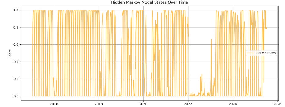
🔌 QuantHQ API Integration: Regime Detection via HMM

This code connects to the QuantHQ Hidden Markov Model (HMM) Regime Detection API and visualizes market regime shifts over time.

🧾 What It Does:

Sends a POST request to QuantHQ’s /api/hmm endpoint
Authenticates using your API key (Bearer token in header)
Requests regime data for QQQ from 2015-01-15 to 2025-07-09
Parses the JSON response and extracts relevant fields:
- id, symbol, date, and regime signal (rhoT)
Loads the data into a pandas DataFrame
Converts:
- date → datetime
- signal → numeric HMM regime values (e.g., 0 = bear, 1 = neutral, 2 = bull)
Calls the plot_hmm_state_transitions(df) function to create a clean visual of how market regimes evolve over time


import requests
import pandas as pd

# API call setup
url = "https://quanthq.io/api/hmm"
api_key = "YOUR_API_KEY"  # Replace with your actual key

headers = {
    "Authorization": f"Bearer {api_key}",
    "Content-Type": "application/json"
}

payload = {
    "symbol": "QQQ",
    "startDate": "2015-01-15",
    "endDate": '2025-07-09'
}

response = requests.post(url, headers=headers, json=payload)

if response.status_code == 200:
    raw_data = response.json()

    # Extract just the fields you care about from the nested 'data' object
    # Example if the API returns {"data": [...actual records...]}
    records_raw = raw_data.get("data", [])
    records = []
    for item in records_raw:
        records.append({
            "id": item.get("id"),
            "symbol": item.get("symbol"),
            "date": item.get("date"),
            "signal": item.get("rhoT")
        })


    # Convert to DataFrame
    df = pd.DataFrame(records)

    # Clean data types
    df["date"] = pd.to_datetime(df["date"])
    df["signal"] = pd.to_numeric(df["signal"], errors="coerce")

    print(df.head())  # optional preview

    # Plot HMM state transitions
    plot_hmm_state_transitions(df)

else:
    print(f"API request failed with status {response.status_code}: {response.text}")

📊 Output:

A preview of the processed DataFrame

A time series plot of the regime signal, ideal for identifying trends, volatility clusters, or structural breaks in the market

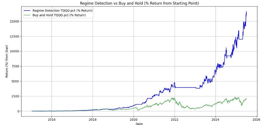
📊 Explosive Backtest Results: TQQQ Strategy Using QQQ Regime Detection

What happens when you apply QuantHQ’s regime detection signal (trained on QQQ) to a leveraged ETF like TQQQ?

✅ Total return: +16,283.12% (Jan 2015–July 2025, simulated)

This isn’t magic — it’s a simple regime-aware overlay. We didn’t tweak parameters, curve-fit, or optimize for hindsight. We just followed this logic:

df['position'] = np.where(df['signal'] > 0.6, 1, 0)

When the Hidden Markov Model (HMM) gives a strong bull signal, we take a position. Otherwise, we sit in cash.

💡 Strategy Overview

Signal source: QQQ (NASDAQ-100)
Traded asset: TQQQ (3x leveraged version of QQQ)
Approach: Only enter when bull regime probability > 60%
No leverage added (TQQQ is already 3x leveraged)

Backtest period: 2015-01-15 to 2025-07-09

import numpy as np
import pandas as pd
import yfinance as yf
import matplotlib.pyplot as plt


# --- Step 1: Fetch price data from Yahoo Finance ---
def get_yfinance_data(symbol: str, start: str, end: str) -> pd.DataFrame:
    df = yf.download(symbol, start=start, end=end, auto_adjust=False)


    if isinstance(df.columns, pd.MultiIndex):
        df.columns = ['_'.join(col).strip() if col[1] else col[0] for col in df.columns.values]


    df = df.reset_index()
    if 'date' not in df.columns and 'Date' in df.columns:
        df.rename(columns={'Date': 'date'}, inplace=True)

    # Try to find the close column smartly (case insensitive)
    close_col = None
    for col in df.columns:
        if col.lower().startswith('close'):
            close_col = col
            break

    if close_col is None:
        raise KeyError("No 'close' column found in yfinance data!")

    df = df[['date', close_col]].rename(columns={close_col: 'close'})
    df['date'] = pd.to_datetime(df['date'])
    return df




# --- Step 2: Backtest using HMM signal ---
def backtest_from_signal(signal_df: pd.DataFrame, price_df: pd.DataFrame, transaction_cost: float = 0.001) -> pd.DataFrame:
    # Reset MultiIndex if present
    if isinstance(signal_df.index, pd.MultiIndex):
        signal_df = signal_df.reset_index()
    if isinstance(price_df.index, pd.MultiIndex):
        price_df = price_df.reset_index()

    # Ensure 'date' is a datetime column with no timezone
    signal_df['date'] = pd.to_datetime(signal_df['date']).dt.tz_localize(None)
    price_df['date'] = pd.to_datetime(price_df['date']).dt.tz_localize(None)

    # Now merge on 'date'
    df = pd.merge(price_df, signal_df[['date', 'signal']], on='date', how='inner')

    df['log_return'] = np.log(df['close'] / df['close'].shift(1))
    df.dropna(inplace=True)

    df['signal'] = df['signal'].shift(1).fillna(0)
    df['position'] = np.where(df['signal'] > 0.6, 1, 0)

    df['strategy_return'] = df['position'] * df['log_return']
    df['trade'] = df['position'].diff().abs().fillna(0)
    df['strategy_return_net'] = df['strategy_return'] - df['trade'] * transaction_cost
    df['equity'] = np.exp(df['strategy_return_net'].cumsum())

    return df[['date', 'close', 'signal', 'position', 'log_return', 'strategy_return_net', 'equity']]


# --- Step 3: Plot the equity curve and closing price ---
def plot_equity(df: pd.DataFrame):
    fig, ax = plt.subplots(figsize=(12, 6))

    df['equity_pct'] = (df['equity'] / df['equity'].iloc[0] - 1) * 100
    df['close_pct'] = (df['close'] / df['close'].iloc[0] - 1) * 100

    ax.plot(df['date'], df['equity_pct'], label='Regime Detection TQQQ pct (% Return)', color='blue')
    ax.plot(df['date'], df['close_pct'], label='Buy and Hold TQQQ pct (% Return)', color='green', alpha=0.6)

    ax.set_xlabel("Date")
    ax.set_ylabel("Return (%) from Start")
    ax.grid(True)
    ax.legend(loc="upper left")
    plt.title("Regime Detection vs Buy and Hold (% Return from Starting Point)")
    plt.tight_layout()
    plt.show()


# --- Step 4: Drawdown calculation ---
def calculate_drawdown(returns):
    cumulative_returns = (1 + returns).cumprod()
    peak = cumulative_returns.expanding(min_periods=1).max()
    drawdown = (cumulative_returns / peak) - 1
    return drawdown


def plot_underwater(strategy_df: pd.DataFrame):
    if 'date' in strategy_df.columns:
        strategy_df['date'] = pd.to_datetime(strategy_df['date'])
        strategy_df = strategy_df.set_index('date')
    elif not isinstance(strategy_df.index, pd.DatetimeIndex):
        print("Warning: DataFrame index is not datetime. Attempting to convert.")
        strategy_df.index = pd.to_datetime(strategy_df.index)

    equity_returns = strategy_df['equity'].pct_change().dropna()
    close_returns = strategy_df['close'].pct_change().dropna()

    equity_drawdown = calculate_drawdown(equity_returns)
    close_drawdown = calculate_drawdown(close_returns)

    fig, ax = plt.subplots(figsize=(12, 6))
    ax.fill_between(equity_drawdown.index, equity_drawdown, 0, color='tab:blue', alpha=0.6, label='Regime Detection Drawdown')
    ax.fill_between(close_drawdown.index, close_drawdown, 0, color='tab:orange', alpha=0.6, label='Buy and Hold Drawdown')

    plt.title("Manual Underwater Plot: Regime Detection vs. Buy and Hold Price Drawdowns")
    plt.xlabel("Date")
    plt.ylabel("Drawdown")
    plt.grid(True)
    plt.legend()
    plt.show()


# --- Step 5: Run the backtest pipeline using yfinance ---
def run_pipeline(signal_df: pd.DataFrame, symbol: str, start: str, end: str):
    # Flatten signal_df index if needed
    if isinstance(signal_df.index, pd.MultiIndex):
        signal_df = signal_df.reset_index()

    price_df = get_yfinance_data(symbol, start, end)
    equity_df = backtest_from_signal(signal_df, price_df)
    plot_equity(equity_df)
    plot_underwater(equity_df)
    final_equity = equity_df['equity'].iloc[-1]
    total_return = final_equity / equity_df['equity'].iloc[0] - 1
    print(f"✅ Final equity: {final_equity:.2f} | Total return: {total_return:.2%}")
    return equity_df

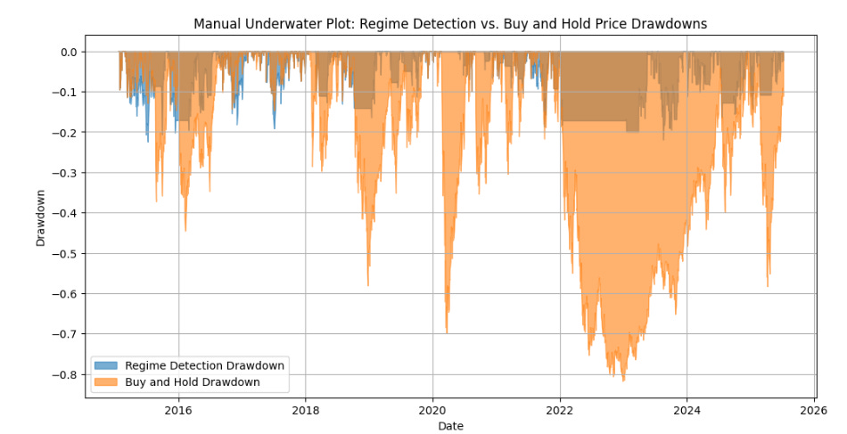
📉 Dramatic Drawdown Reduction

One of the key benefits wasn’t just return — it was risk reduction:

✅ Drawdowns are significantly lower than buy-and-hold TQQQ
✅ The strategy exits during weak regimes, avoiding major crashes
✅ Equity curve is smoother and more compounding-friendly

We visualized this in a custom underwater plot to compare strategy vs. passive investing — the difference is stark.

🛑 Important Disclaimer

⚠️ Backtested results are not guarantees of future performance. This strategy uses historical data and should be viewed as a research demonstration only. Leveraged ETFs like TQQQ are inherently risky and may not be suitable for all investors. Always do your own due diligence and consider speaking with a financial advisor.

✅ Why Now Is the Perfect Moment to Subscribe

You’ve just seen impressive historical results, including:

Annual return of 62.98% (based on backtested data)
Sharpe ratio of 1.74 (indicating strong risk-adjusted performance)
Max drawdown limited to -22.44%
Cumulative returns of over 16,000% across the backtest period

While past performance is not a guarantee of future results, these metrics highlight the potential value of quantitative regime detection strategies.

This is a great opportunity to stay informed and deepen your understanding of these approaches.

🔥 What You’ll Receive When You Subscribe

Early access to new strategy backtests and research, delivered before public release
Educational content on advanced quant models and market regime insights
Thoughtful analysis designed to help you better understand risk and opportunity
Updates on new tools and APIs to support your quant trading journey

📩 Interested in receiving actionable quant insights?

👉 Subscribe to the free QuantHQ Newsletter and get fresh analysis and strategy ideas delivered directly to your inbox.

Please remember: This newsletter is for educational purposes only and does not constitute financial advice or an offer to trade securities.

Intrinsic Research

Discussion about this post